Tutorial on MD Simulations

This webpage aims to serve as an archive to help me do MD simulations. Detailed procedures of preparing model and performing MD are illustrated. Three examples are included: adenylate kinase (AdK) for MD and well-tempered metaD, liganded protein for modelling drug-protein complex, and a prototypical example of a receptor protein in a lipid bilayer. I have gone through every step to make sure it works. I hope these examples can be modified to fit to your need.

Adenylate kinase in an aqueous solution


Adenylate kinase (AdK) is the key enzyme in maintaining the cellular energy homeostasis. AdK comprises three relatively rigid domains, central core (CORE), an AMP-binding domain (AMPbd), and a lid-shaped ATP-binding domain (ATPlid). During the catalytic cycle of AdK, the largest conformational changes occur in the ATPlid and the AMPbd domains, while the CORE remains relatively unchanged. During the catalytic reaction, several metastable configurations exist to bridge the open and closed states of the enzyme. Here we describe the molecular dynamic (MD) simultion procedure of AdK with Gromacs 5.1.2 and Plumed 2.2. First we will show how to prepare the files needed for the simulation and how to analyze the MD trajectories. We will also show the detailed step to extract free energy profile with metadynamics by combining Gromacs and Plumed.

Regular Molecular Dynamic Simulation

A. Prepare the Structural and Topological Files of the Protein

In the folder of working space, I will create an AdK folder for this simulation. In the AdK folder, for the concern of organized data, it is helpful to create some other subfolders: coord (pdb, etc.), mdp (input parameters for md run), md (md run), WTmetaD, etc.
  $ mkdir AdK | cd AdK
  $ mkdir coord mdp md top WTmetaD
  $ cd coord
  $ wget http://www.rcsb.org/pdb/files/3adk.pdb

Next, we have to fix the errors or missing residues of the pdb file using the handy online tool "pdbfixer":
  $ cd ~/pdbfixer
  $ pdbfixer

On the "Welcome To PDBFixer!" page, input your 3adk.pdb file and hit "Analyze file" button. This PDB file contains 2 chains. Select chain #1 (Protein, 195 residues) to be included. Hit "Continue" button. Delete all heterogens atoms (except amino acid residues and nuclei acids). Do not add missing Hydrogens. Deselect "Add water" and then hit "Continue" button. Save the fixed file!

Next, we will prepare the structure, topology (.top) and relevant topology include file (.itp) using the pdb file. Three new files will be generated: adk.gro, adk.top, and adk_posre.itp from pdb2gmx.
adk.gro output (-o) is a gro-formatted structure file that contains all the atoms' coordiates defined in the force field.
The .top file (-p) is the system topology.
The .itp file (-i) contains information used to restrain the positions of heavy atoms.
Choose force field charmm27. The protein (23582 amu) possesses -4e charges. For help, type: gmx_mpi help pdb2gmx. Go back to AdK folder.
  $ cd top
  $ gmx_mpi pdb2gmx -f ../coord/3adk.pdb -o adk.gro -p adk.top -i adk_posre.itp -water tip3p -ff charmm27 -nochargegrp -ignh

B. Prepare a Simulation Box, Solvate the Protein and Neutralize the Simulation System

Generate a simulation box and center (-c) the protein in the box using editconf, which needs the processed protein structural file .gro. Allow at least 1.0 nm (-d 1.0) from the rim of the protein to the boundary of the cubic box (-bt cubic).
  $ cd ../md
  $ gmx_mpi editconf -f ../top/adk.gro -c -d 1.0 -bt cubic -o adk_box.gro
gmx_mpi solvate: Add in solvent molecules (water) to the simulation box.
Note: adk.top will be modified and adk_sol.gro will be generated. The configuration of the protein (-cp) is contained in adk_box.gro, and the configuration of the solvent (-cs) is part of the standard GROMACS installation. adk.top (-p) will be modified to include topology information of solvent molecules.
  $ gmx_mpi solvate -cp adk_box.gro -cs -p ../top/adk.top -o adk_sol.gro

The output of pdb2gmx told us that the protein has a net charge of -4e. To neutralize the charges, we prepare the needed ions topology file (-o .tpr) by using grompp with parameters included with (-f ions.mdp), (-c) coordinates and (-p) topology information.
Use this ion.mdp file to prepare .tpr file for genion.
  $ gmx_mpi grompp -f ../emin/ion.mdp -p ../top/adk.top -c adk_sol.gro -o adk_ions.tpr -maxwarn 3
  $ echo "SOL" | gmx_mpi genion -s adk_ions.tpr -pname NA -nname CL -conc 0.1 -neutral -p ../top/adk.top -o adk_ions.gro

C. Relax Solvent Configuration with Energy Minimization

This will relax the solvent structure and ions through an energy minimization process while fix the protein position. The following files will be produced:
adk_em.log, adk_em.edr (binary energy file), adk_em.trr (binary full-precision trajectory), adk_em.gro (energy-minimized structure).
Use this em.mdp file to prepare .tpr file for energy minimization.
  $ gmx_mpi grompp -f ../mdp/em.mdp -c adk_ions.gro -p ../top/adk.top -o adk_em.tpr -maxwarn 3
  $ gmx_mpi mdrun -v -s adk_em.tpr -deffnm adk_em -c adk_em.pdb
  $ gmx_mpi energy -f adk_em.edr -o Epot.xvg
Select 11 for output Potential.
  $ xmgrace Epot.xvg

3D model of AK1

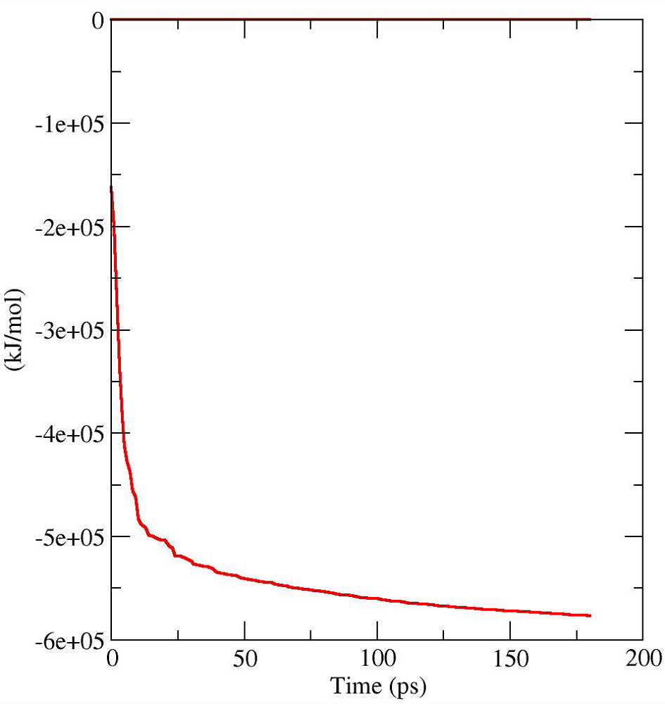
FIG.1: Time course of potential energy in an energy minimization run.

D. Equilibrate the System

Using the energy-minimization structure (-c) adk_em.pdb as an input, first perform a NVT MD run to equilibrate the system at a given temperature.
Use this nvt.mdp file to prepare .tpr file for nvt equilibration.
  $ gmx_mpi grompp -maxwarn 2 -f ../mdp/nvt.mdp -c adk_em.pdb -p ../top/adk.top -o adk_nvt.tpr
  $ gmx_mpi mdrun -v -s adk_nvt.tpr -deffnm adk_nvt
  $ gmx_mpi energy -f adk_nvt.edr -o adk_T.xvg
Select 16 to output Temperature.
  $ xmgrace adk_T.xvg

3D model of AK1

FIG.2: Time course of system temperature in a NVT run.

Check that the system was brought up to 300K.

Using the NVT equilibrated structure as an input, continue to perform a NPT MD run to equilibrate the system at a given pressure. The MD run starts with the previous nvt MD result (-c adk_nvt.gro -t adk_nvt.cpt). Use this npt.mdp file to prepare .tpr file for the npt equilibration.
  $ gmx_mpi grompp -maxwarn 2 -f ../mdp/npt.mdp -c adk_nvt.gro -t adk_nvt.cpt -p ../top/adk.top -o adk_npt.tpr
  $ gmx_mpi mdrun -v -s adk_npt.tpr -deffnm adk_npt
  $ gmx_mpi energy -f adk_npt.edr -o adk_P.xvg
Select 17 to output pressure.
  $ xmgrace adk_P.xvg
  $ gmx_mpi energy -f adk_npt.edr -o adk_d.xvg
Select 23 to output density.
  $ xmgrace adk_d.xvg

3D model of AK1

FIG.3: Time course of total density in a NPT run.

Check that the pressure fluctuates randomly at 1 bar; the density fluctuates weakly at 1017 kg/m3

E. Production MD Run

Run a 2-ns production MD using an input structure from adk_npt.gro and full precision trajectory file (-t .cpt) from npt run. Use this md.mdp file to prepare .tpr file for a production MD run.
  $ gmx_mpi grompp -f ../mdp/md.mdp -c adk_npt.gro -t adk_npt.cpt -p ../top/adk.top -o adk_md.tpr -maxwarn 2
  $ gmx_mpi mdrun -v -s adk_md.tpr -deffnm adk_md

F. Trajectory Analysis with bio3D

I. Prepare structural (adk_md.tpr) and trajectory files (adk_md.xtc) for bio3d analysis
Extract the protein (-pbc mol) from the first frame (-dump 0) of the trajectory file (adk_md.xtc). Then, extract (-pbc mol) and center (-center) the protein trajectory.
  $ gmx_mpi trjconv -s adk_md.tpr -f adk_md.xtc -o adk_md.gro -pbc mol -ur compact -center -dump 0
  $ gmx_mpi trjconv -s adk_md.tpr -f adk_md.xtc -o adk_md_nPBC.xtc -pbc mol -ur compact -center

Convert .xtc trajectory to .dcd
  $ mdconvert adk_md_nPBC.xtc -t adk_md.gro -o adk_md.dcd
The two files needed for bio3d analysis: adk_md.pdb adk_md.dcd (501 frames) with 4 ps frame time.

II. Trajectory Analysis with bio3d---Launch and Data Input
  $ sudo R
  > library(bio3d)
  > pdb<-read.pdb("adk_md.pdb")
  > dcd<-read.dcd("adk_md.dcd", cell=FALSE)
  NATOM = 41060
  NFRAME= 101
  ISTART= 0
  last = 101
  nstep = 101
  nfile = 101
  NSAVE = 1
  NDEGF = 0
  version 24

  > ca.inds<-atom.select(pdb,"protein",elety="CA")
  > trj<-fit.xyz(pdb$xyz, dcd, fixed.inds=ca.inds$xyz, mobile.inds=ca.inds$xyz)
  > protpdb<-trim.pdb(pdb,ca.inds)
  > protdcd<-trim(trj, col.inds=ca.inds$xyz)
  > print(protpdb$xyz)
  Total Frames#: 1
  Total XYZs#: 582, (Atoms#: 194)
   [1] 40.231 33.421 13.441 <...> 21.171 32.731 20.411 [582]
  + attr: Matrix DIM = 1 x 582

  > print(protdcd)
  Total Frames#: 101
  Total XYZs#: 582, (Atoms#: 194)
  [1] 40.231 33.421 13.441 <...> 21.626 33.99 20.425 [58782]
  + attr: Matrix DIM = 101 x 582

III. Trajectory Analysis with bio3d---RMSD
  > rd<-rmsd(protpdb, protdcd, fit=TRUE, ncore=4)
  > plot(rd,typ="l",ylab="RMSD",xlab="Frame No.")
  > points(lowess(rd), typ="l", col="red", lty=1, lwd=3)
  > dev.copy(jpeg,filename="adk_rmsd.jpg")
  > dev.off()

3D model of AK1

FIG.4: RMSD of AdK structure plotted as a function of frame number (with a frame time of 4 ps).

  > rf<-rmsf(protdcd)
  > plot(rf,ylab="RMSF",xlab="Residue Position",typ="l")
  > dev.copy(jpeg,filename="adk_rmsf.jpg")
  > dev.off()

FIG.5: RMSF Analysis revealing the fluctuating residues of the protein.

  > pc<-pca.xyz(protdcd)
  > plot(pc,col=bwr.colors(nrow(dcd)))
  > dev.copy(jpeg,filename="adk_pca.jpg")
  > dev.off()

FIG.6: PCA Analysis revealing the most significant collective motions. The first three PCAs contribute 52% fluctuation of the protein.

  > plot.bio3d(pc$au[,1],ylab="PC1(Blue), PC2(Red)",xlab="Residue Position", typ="l",col="blue",lty=1,lwd=3)
  > points(pc$au[,2],typ="l",col="red",lty=1,lwd=3)
  > dev.copy(jpeg,filename="adk_pcs2resid.jpg")
  > dev.off()

FIG.7: Two most significant PCA components are decomposed into the RMSFs of each residue.

IV. Trajectory Analysis with bio3d---Normal Mode Analysis (NMA)
  > pdb <- read.pdb("adk_md.pdb")
  > dcd <- read.dcd("adk_md1.dcd", cell=FALSE)
  > prot.inds <- atom.select(pdb,"protein")
  > trj <- fit.xyz(pdb$xyz, dcd, fixed.inds=prot.inds$xyz, mobile.inds=prot.inds$xyz)
  > protpdb <- trim.pdb(pdb,prot.inds)
  > protdcd <- trim(trj, col.inds=prot.inds$xyz)
  > modes <- nma(protpdb)
   Building Hessian... Done in 0.039 seconds.
   Diagonalizing Hessian... Done in 0.258 seconds.
  > cij <- dccm(modes, ncore=4)
  > net <- cna(cij, cutoff.cij=0.3, ncore=4)
  > print(net)
   Call: cna.dccm(cij = cij, cutoff.cij = 0.3, ncore = 4)
   Structure:
   - NETWORK NODES#: 194 EDGES#: 848
   - COMMUNITY NODES#: 11 EDGES#: 20
   + attr: network, communities, community.network,
   community.cij, cij, call

  > x <- summary(net)
   id  size   members
   1   8   1:8 (core)
   2   25   c(9:14, 34:38, 87:95, 112:116) (core)
   3   14   c(15:17, 19, 117:120, 172:177) (core)
   4   18   c(18, 121:132, 134:138) (lid)
   5   14   20:33 (core)
   6   31   c(39:67, 133, 145) (nmp)
   7   19   68:86 nmp-core)
   8   15   c(96, 98:111) (core)
   9   26   c(97, 147:171) (core)
   10   7   c(139:144, 146) (lid)
   11  17  178:194 (core)

   Note: Core: 1-16, 19-38, 77-120, 153-194; Lid: 121-152; NMP: 39-76

  > plot(net, protpdb)
  > dev.copy(jpeg,filename="adk_net.jpg")
  > dev.off()

FIG. 8: Graph (deduced from normal mode analysis) showing coupling between different domains (nmp, lid and core) of AdK.

G. Determine the rigid domains of 3ADK Protein Structure

Go to the website of "http://pisqrd.escience-lab.org/"
  a. Browse to the file position of 3ADK and Hit the "Submit Calculation" button.
  b. Wait for the result.
   The minimum number of domains needed to capture >80 % of the internal essential dynamics: 3
   Hit "View Protein Subdivision (opens in new page)" and save the page into a text file.

FIG. 9: Model showing three different domains (core: blue and gray, lid: green, and nmp: red) of AdK.

Well-Tempered Metadynamics Simulation

A. Prepare the Structural/Topological Files and Perform a Unbiased MD Run

Go to the folder of Adk working space. Perform a unbiased MD run.
  $ cd WTmetaD
  $ gmx_mpi grompp -f ../mdp/md.mdp -c ../md/adk_md.gro -p ../top/adk.top -o adk_md.tpr -maxwarn 2
  $ gmx_mpi mdrun -v -s adk_md.tpr -deffnm adk_unbiased -plumed plumed_unbiased.dat

Do the following analysis:
1. Plot the time dependence of theta1, theta2, and disln in the unbiased run
  $ gnuplot
  gnuplot> set datafile commentschars "#!"
  gnuplot> set xlabel "time (ps)"
  gnuplot> set ylabel "theta1 theta2 (rad)"
  gnuplot> plot "colvar" u 1:2 t 'theta1' w lp lc 3 lw 2, "colvar" u 1:3 t 'theta2' w lp lc 1 lw 2
  gnuplot> set terminal jpeg
  gnuplot> set output "unbiased-theta_traj.jpg"
  gnuplot> replot
  gnuplot> q

B. WTmetaD

In the WTmetaD folder, perform a well-tempered metadynamics MD run using this plumed.dat file.
  $ gmx_mpi mdrun -v -s adk_md.tpr -deffnm adk_metad -plumed plumed.dat
  $ ls
  --> colvar HILLS adk_metad.cpt adk_metad.edr adk_metad.gro adk_metad.log adk_metad.trr adk_metad.xtc
Do the following analysis:
1. Plot the time dependence of theta1, theta2, and disln in the unbiased run
  $ gnuplot
  gnuplot> set datafile commentschars "#!"
  gnuplot> set xlabel "time (ps)"; set ylabel "theta1 theta2 (rad)"
  gnuplot> plot[1:6000] "colvar" u 1:2 t 'theta1' w lp lc 3 lw 1, "colvar" u 1:3 t 'theta2' w lp lc 1 lw 1
  gnuplot> set term jpeg
  gnuplot> set output "biased-theta_traj.jpg"
  gnuplot> replot
  gnuplot> set output "Hills_traj.jpg"
  gnuplot> set xlabel "time (ps)"; set ylabel "Hills (kJ/mol)"
  gnuplot> plot "HILLS" u 1:6 t 'Gaussian height' w linespoints lt 1 lc 1 lw 1
  gnuplot> set term wxt 1
  gnuplot> q

FIG. 10: Hills added as WTmetaD of AdK.

2. Free Energy Mapping
  $ plumed sum_hills --hills HILLS
  --> fes.dat
  $ gnuplot
  gnuplot> set pm3d map
  gnuplot> splot "fes.dat"
  gnuplot> set terminal jpeg
  gnuplot> replot
  gnuplot> q

FIG. 11: Free energy surface of AdK on theta1 and theta2

3. Calculate one-dimensional free energies from the two-dimensional metadynamics simulation
  $ plumed sum_hills --hills HILLS --idw theta1 --kt 2.5 --stride 2000 --outfile fes_proj_theta1 --mintozero
  $ plumed sum_hills --hills HILLS --idw theta2 --kt 2.5 --stride 2000 --outfile fes_proj_theta2 --mintozero
  $ gnuplot
  gnuplot> set grid; set autoscale fix
  gnuplot> set title 'Free Energy Projection on theta1'
  gnuplot> set xlabel 'theta1'; set ylabel 'FE (kcal/mol)'
  gnuplot> unset key
  gnuplot> plot 'fes_proj_theta11.dat' u 1:($2*0.2388) w l lt 1 lc 1 lw 1,'fes_proj_theta13.dat' u 1:($2*0.2388) w l lt 1 lc 3 lw 1
  gnuplot> set terminal jpeg
  gnuplot> set output "fes-theta1_3adk.jpg"
  gnuplot> replot
  gnuplot> set output "fes-theta2_3adk.jpg"
  gnuplot> set title 'Free Energy Projection on theta2'
  gnuplot> set xlabel 'theta2'; set ylabel 'FE (kcal/mol)'
  gnuplot> plot 'fes_proj_theta21.dat' u 1:($2*0.2388) w l lt 1 lc 1 lw 1,'fes_proj_theta23.dat' u 1:($2*0.2388) w l lt 1 lc 3 lw 1
  gnuplot> q

FIG. 12: Free energy of AdK projection on (left) theta1 and (right) theta2.

Liganded Protein


A longstanding goal in structure based drug discovery is to predict ligand binding free energies accurately. In this regards, T4 Lysozyme complexed with 2-propylphenol serves as a prototypical example for calculating the absolute binding free energy of different compounds to the hydrophobic model binding site. This example aims to illustrate how to prepare a complex model of a protein (T4 Lysozyme) with a ligand (2-propylphenol) for MD simulation.

A. Prepare the Structure and Topological File of the Complex

In the folder of working space, first I created an AdK folder for this simulation. In this AdK folder, I also created some subfolders to organize data: coord (pdb, etc.), mdp (input parameters for md run), and md (md run), etc.
  $ mkdir LigProtein | cd LigProtein
  $ mkdir coord mdp md top
  $ cd coord
  $ wget http://www.rcsb.org/pdb/files/3HTB.pdb
  $ grep "JZ4" 3HTB.pdb > Lig.pdb

Next, we select the protein and fix the missing residues of the pdb file using the handy online tool "pdbfixer":
  $ cd ~/pdbfixer
  $ pdbfixer

On the "Welcome To PDBFixer!" page, input your 3HTB.pdb file and hit "Analyze file" button. This PDB file contains 1 protein chain and JZ4 ligand. Select chain #1 (the protein) to be included. Hit "Continue" button. Delete all heterogens atoms (except amino acid residues and nuclei acids). Do not add missing Hydrogens. Deselect "Add water" and then hit "Continue" button. Save the fixed file as Prot.pdb!

Next, we will prepare the structure and topology of JZ4 compound. However, some hydrogen atoms are missing in JZ4.pdb, so we use obabel to insert the missing H atoms (-h) to JZ4.pdb (-ipdb) and then output as mol2 format (-omol2):
  $ obabel -h -ipdb Lig.pdb -omol2 -O JZ4.mol2
Submit JZ4.mol2 to SwissParam to create a topology file of JZ4. Download the zip file and uncompress it to retrieve JZ4.itp and JZ4.pdb. Rename the ligand name from LIG to JZ4 with:
  $ sed -i "s/LIG/JZ4/g" JZ4.pdb

Prepare the topology .top and coordinates file conf.pdb of the protein (without ligand).
  $ gmx_mpi pdb2gmx -f Prot.pdb -o conf.pdb -p ../top/Prot.top -water tip3p -ff charmm27 -nochargegrp -ignh

B. Prepare the Complex

  $ cd ../top
  $ nano Prot.top
Modify protein's topology file (Prot.top) as follow:
   ; Include forcefield parameters
    #include "charmm27.ff/forcefield.itp"
    #include "JZ4.itp"

Place include file (#include "JZ4.itp") diretly behind the forcefield include file, but before any [ moleculetype ]. This statement has to be at this precise position in the file because that JZ4.itp includes [atomtypes] directive, which will need some forcefield information. Violate this rule will generate an error of "Invalid order for directive atomtypes". Then, right after lines indicating the number of protein molecules, add "JZ4 1" in the [ molecules ] section:
    [ molecules ]
    ; Compound    #mols
    Protein_chain_A   1
    JZ4        1

If there are crystal water molecules in the structure, there will be a line indicating the number of solvent molecules (SOL) in the topology. In this case, the line above should be inserted before any SOL and ions lines. See below for an example Prot.top file. Name the new topol file as "complex.top" and stores it in the folder of "./top/".
Merge the protein and ligand coordinates. Insert the ATOM lines from the JZ4.pdb into the conf.pdb file, right after the line of the last residue of the protein. Atoms will be automatically renumbered in the next step. Name the new file as complex.pdb.

C. Gromacs Setup Procedure

Now we are back to the usual GROMACS setup procedure. Up one level to the folder of ./LigProtein:
  $ cd ..
  $ gmx_mpi editconf -f ./coord/complex.pdb -o ./coord/complex_boxed.gro -p ./top/complex.top -c -d 1.2 -bt octahedron
  $ gmx_mpi solvate -cs -cp ./coord/complex_boxed.gro -o ./coord/complex_solvated.gro -p ./top/complex.top
If you have an appropriate input file em.mdp for an energy minimization in GROMACS, you can then run
  $ gmx_mpi grompp -f ./mdp/em.mdp -c ./coord/complex_solvated.gro -p ./top/complex.top -o ./md/complex_solvated.tpr
  $ echo "SOL" | gmx_mpi genion -s ./md/complex_solvated.tpr -pname NA -nname CL -conc 0.1 -neutral -p ./top/complex.top -o ./coord/complex_ions.gro -maxwarn 2
It is possible to include position restraints on the ligand by using the POSRES_LIGAND flag. In the case where both protein and ligand atoms should be restrained, the corresponding line in the em.mdp file would read:
   define = -DPOSRES -DPOSRES_LIGAND

Notes:
To verify that your solvated molecule looks good in its octahedric box, you have to remember that Gromacs always works internally with an equivalent triclinic unit cell. To see the octahedron, you will have to transform your coordinates (after having run grompp), using:
  $ gmx_mpi trjconv -s ./md/complex_solvated.tpr -f ./coord/complex_solvated.gro -o ./coord/compact.pdb -ur compact -pbc mol
  $ vmd compact.pdb

FIG.2: Model of JZ4(red)-T4 lysozyme (coloring by residue type) complex .

D. Relax SOL/Ions Positions with Energy Minimization

Now we first to relax the solvent molecules and ions with a fixed protein using energy minimization procedure:
  $ gmx_mpi grompp -f ./mdp/em.mdp -c ./coord/complex_ions.gro -p ./top/complex.top -o ./md/complex_em.tpr
  $ gmx_mpi mdrun -v -s ./md/complex_em.tpr -deffnm ./md/complex_em -c ./coord/complex_em.pdb

E. Equilibrate the System

Applying restraints to the ligand. In the nvt.mdp, set
   tc_grps = Protein_JZ4 Water_and_ions
to achieve our desired "Protein Non-Protein" effect.
  $ gmx_mpi genrestr -f ./Lig/JZ4.gro -o ./top/posre_JZ4.itp -fc 1000 1000 1000

Treatment of temperature coupling groups by combining 1 (protein) and 13 (JZ4) as one group: 1 | 13
  $ gmx_mpi make_ndx -f ./coord/complex_em.pdb -o ./coord/index.ndx
Proceed with NVT equilibration
  $ gmx_mpi grompp -f ./mdp/nvt.mdp -c ./coord/complex_em.pdb -p ./top/complex.top -n ./coord/index.ndx -o ./md/complex_nvt.tpr
  $ gmx_mpi mdrun -v -s ./md/complex_nvt.tpr -deffnm ./md/complex_nvt -c ./coord/complex_nvt.pdb

Continue to NPT run:
  $ gmx_mpi grompp -f ./mdp/npt.mdp -c ./coord/complex_nvt.pdb -p ./top/complex.top -n ./coord/index.ndx -o ./md/complex_npt.tpr
  $ gmx_mpi mdrun -v -s ./md/complex_npt.tpr -deffnm ./md/complex_npt -c ./coord/complex_npt.pdb

F. Perform a Production MD

Run a 1-ns production MD simulation
  $ gmx_mpi grompp -f ./mdp/md.mdp -c ./coord/complex_npt.pdb -p ./top/complex.top -n ./coord/index.ndx -o ./md/complex_md1.tpr
  $ gmx_mpi mdrun -v -s ./md/complex_md1.tpr -c ./coord/complex_npt.pdb -deffnm ./md/complex_md1

EGFR Dimer in a Lipid Bilayer


The epidermal growth factor receptor (EGFR) is a transmembrane protein, which contains an extracellular binding domain, a single transmembrane spanning domain, and a cytoplasmic tyrosine kinase domain. Ligands bind to the extracellular domain of EGFR, stimulating conformational changes that support receptor dimerization. Receptor dimerization leads to the activation of the intracellular tyrosine kinase domain and phosphorylates the dimerization partner on specific tyrosine residues. The phosphorylated tyrosine residues then function as docking sites for adaptor proteins, which further activate intracellular signaling cascades. This example aims to illustrate how to prepare a model of a membrane protein (EGFR dimer) embedded in a lipid bilayer for MD simulation. To simplify the simulation only the transmembrane spanning domain of EGFR is included.

[I]. Prepare Gromacs Forcefield for Lipids

The Gromacs pdb2gmx engine can only process proteins, nucleic acids, ions and a few co-factors. We need to manually add the topology of POPC to the force-field topology files. However, if using CHARMM36 FF, then no need to modify the contents of the bonded.itp and nonbonded.itp files, as CHARMM36 already includes parameters for some of the commonly used lipid molecules like POPC.

Prepare Gromacs forcefield for lipids by including lipid.itp file:
  $ cd ~/
  $ mkdir gromos53a6_lipids.ff
Copy atomtypes.atp aminoacids.rtp, aminoacids.hdb, aminoacids.c.tdb, aminoacids.n.tdb, aminoacids.r2b, aminoacids.vsd, ff_dum.itp, ffnonbonded.itp, ffbonded.itp, forcefield.itp, ions.itp, spc.itp and watermodels.dat files from /opt/Gromacs/share/gromacs/top/gromos53a6.ff to this folder.

You will need popc.itp and lipid.itp, which can be downloaded from here. Copy the entries under the [ atomtypes ], [ nonbond_params ], and [ pairtypes ] sections from "lipid.itp" file and paste them into the appropriate headings within the "ffnonbonded.itp" file. Delete all the lines under the section [ nonbond_params ] starting from the line
" ; ; parameters for lipid-GROMOS interactions."
till the end of the section. Now, add the contents under the [ dihedraltypes ] section from the lipid.itp file to the corresponding section of "ffbonded.itp" file.
  $ sudo mv ~/gromos53a6_lipids.ff /opt/Gromacs/share/gromacs/top/

[II]. Prepare folders and relevant Gromacs files needed MD

Using the following cmdline scripts:
  $ cd ~/
  $ mkdir hEGFR2
  $ cd hEGFR2
  $ mkdir coord mdp md top
  $ cd coord

1. Download protein pdb file from RCSB PDB:
  $ wget http://www.rcsb.org/pdb/files/2M20.pdb
2. fix the file with pdbfixer
  $ cd ~/pdbfixer
  $ pdbfixer
Browser to the file of 2M20.pdb, analyze the file. Select both chains, keep heteroatoms and all hydrogen atoms (pH=7) without adding water. Save the file (output.pdb) and quit.
  $ mv ~/pdbfixer/output.pdb ~/hEGFR2/coord/2M20_fixed.pdb
3. Prepare relevant files for Gromacs:
  $ cd ~/hEGFR2/coord
  $ gmx_mpi pdb2gmx -f 2M20_fixed.pdb -merge all -o hEGFR2.gro -p ../top/topol.top -i ../top/posre -ignh -ter -water spc
Select 15 for GROMOS96 53A6 force field, extended to include Berger lipid parameters;
The option -missing ignores any missing atoms.
Interactively assign charge states for N- and C-termini: choose 1 for all
--> hEGFR2.gro posre.itp topol.top will be generated.

Do the following changes in the top section of the topol.top file:
  $ nano ../top/topol.top

Towards the end of the topol.top file, add the ";Include POPC chain topology" section:
; Include Position restraint file
#ifdef POSRES
#include "../top/posre.itp"
#endif

; Include POPC chain topology
#include "gromos53a6_lipids.ff/popc.itp"

; Include water topology
#include "gromos53a6_lipids.ff/spc.itp"

Under the [ molecules ] section, add
POP 288
to indicate 288 POPC molecules been included.

4. Prepare lipid bilayer
You can prepare a lipid bilayer in this website. Build a solvated POPC bilayer with 144 lipids in each leaflet: popc288.pdb and popc288.top
Move popc288.pdb to the coord folder, and popc288.top to the top folder.
  $ gmx_mpi make_ndx -f popc288.pdb -o popc288.ndx
Select 2 for POP
  $ echo "2 2" | gmx_mpi editconf -f popc288.pdb -n popc288.ndx -o popc288.gro -d 2

  system size : 10.097   9.803   4.259 (nm)
  center   : 7.048    6.902   4.129 (nm)
  box vectors : 14.097  13.803   8.259 (nm)

Generate a .tpr file for a popc-only system using grompp:
  $ touch ../top/popc288.top
Insert the following lines into the file:

; Include chain topologies
#include "gromos53a6_lipids.ff/forcefield.itp"
#include "gromos53a6_lipids.ff/popc.itp"

; Include water topology
#include "gromos53a6_lipids.ff/spc.itp"

; Include ion topologies
#include "gromos53a6_lipids.ff/ions.itp"

; System specifications
[ system ]
288-Lipid POPC Bilayer

[ molecules ]
; molecule name nr.
POP 288

  $ gmx_mpi grompp -f ../mdp/em.mdp -c popc288.gro -p ../top/popc288.top -o ../md/popc288_em.tpr

The .tpr file contains information about bonding and periodicity, so it can be used to reconstruct "broken" molecules.
Use trjconv to remove periodicity by using the following commands:
  $ gmx_mpi trjconv -s ../md/popc288_em.tpr -f popc288.gro -o popc_bilayer.gro -pbc mol -ur compact

Now, take a look at the last line of this popc_bilayer.gro; it corresponds to the x/y/z box vectors of the POPC unit cell:
  $ tail -1 popc_bilayer.gro
--> 14.09700   13.80300   8.25900

[III]. Assemble protein in lipid bilayer system

1. Insert hEGFR2 into the lipid bilayer
First, we need to orient the protein within this same coordinate frame, and place the center of mass of the protein (hEGFR.gro) at the center of this box:
  $ gmx_mpi editconf -f hEGFR2.gro -o hEGFR2_box.gro -box 14.097 13.803 8.259 -center 7.048 6.902 4.129
The center of the hEGFR2 now lies at (7.048 6.902 4.129) of a box.

Then, prepare ndx files for the protein (select 1 for protein) and popc molecules (use 2 for POPC)
  $ gmx_mpi make_ndx -f hEGFR2_box.gro -o hEGFR2.ndx
  $ gmx_mpi make_ndx -f popc_bilayer.gro -o popc288.ndx

2. Orient the protein using LAMBADA
You can download the code from git hub via the command: $ git clone https://github.com/THSchmidt/lambada-align
  $ ~/lambada-align/lambada -f1 hEGFR2_box.gro -f2 popc_bilayer.gro -n1 hEGFR2.ndx -n2 popc288.ndx -v
--> Mapping atoms to the grid: 100%
   Detecting protein internal cavities: 0.1900 nm^2 detected
   Detecting protein surface: 100%
   Found hydrophobic belt (LS = 242.080) at z >= 75.000 and z <= 99.000 (Angstrom)

The combined model of protein and membrane is stored in the output file "prot_memb.gro".
You can visualize the prot_memb.gro structure with vmd:
  $ gmx_mpi grompp -f ../mdp/em.mdp -c prot_memb.gro -p ../top/topol.top -o ../md/protmemb_em.tpr
  $ gmx_mpi trjconv -s ../md/protmemb_em.tpr -f prot_memb.gro -o prot.gro -pbc mol -ur compact
<-- Select 1 for Protein
  $ gmx_mpi trjconv -s ../md/protmemb_em.tpr -f prot_memb.gro -o memb.gro -pbc mol -ur compact
<--Select 13 for POPC

Load both "prot.gro" and "memb.gro" into vmd and select a proper graphical representation.

FIG.1: Model of hEGFR dimer in a POPC bilayer. Here only transmembrane helix and cytoplasma segment of EGFR are displayed.

3. Embedding the Protein in POPC Bilayer with InflateGRO2
You can download the code from git hub via: $ git clone https://github.com/THSchmidt/inflategro2
A. First. modify topol.top file by
  $ nano ../top/topol.top
Add a new line after #include "posre.itp" in topol.top file:

; Strong position restraints for InflateGRO
#ifdef STRONG_POSRES
#include "../top/strong_posre.itp"
#endif

B. Generate this new position restraint file using genrestr:
  $ echo 1 | gmx_mpi genrestr -f hEGFR2_box.gro -o ../top/strong_posre.itp -fc 100000 100000 100000
Add a line "define = -DSTRONG_POSRES" in .mdp to make use of these new position restraints.

C. Follow the InflateGRO instructions (contained in the script itself), a procedure that is easily scripted. Scale the lipid positions by a factor of 4:
  $ perl ~/inflategro2/inflategro.pl prot_memb.gro 1 POP 14 inflated.gro 5 area.dat

Ref: The InflateGRO script requires a very specific order to its cmdline arguments. A brief explanation is described here:
   prot_memb.gro - the input coordinate file name to which scaling will be applied
   4 - the scaling factor to apply. A value > 1 indicates inflation, a value < 1 indicates shrinking/compression
   POP - the residue name of the lipid to which scaling is applied
   14 - the cutoff radius (in ?) for searching for lipids to delete
   inflated.gro - the output file name
   5 - grid spacing (also in ?) for area per lipid calculation
   area.dat - output file with area per lipid information, useful in assessing the suitability of the structure

--> Reading.....
Scaling lipids....
There are 288 lipids...
with 52 atoms per lipid..

Determining upper and lower leaflet...
144 lipids in the upper...
144 lipids in the lower leaflet
Centering protein....
Checking for overlap....
...this might actually take a while....
100 % done...
There are 37 lipids within cut-off range...
16 will be removed from the upper leaflet...
21 will be removed from the lower leaflet...
Writing scaled bilayer & centered protein...

Calculating Area per lipid...
Protein X-min/max: 51   101
Protein Y-min/max: 55   83
X-range: 50 A   Y-range: 28 A
Building 50 X 28 2D grid on protein coordinates...
Calculating area occupied by protein..
full TMD..
upper TMD....
lower TMD....
Area per protein: 6 nm^2
Area per lipid: 1.50263658167331 nm^2

Area per protein, upper half: 3 nm^2
Area per lipid, upper leaflet : 1.4967257109375 nm^2

Area per protein, lower half: 5.5 nm^2
Area per lipid, lower leaflet : 1.53724301626016 nm^2

Writing Area per lipid...
Done!

D. Slowly pack the lipids around the protein till the area per lipid becomes around 65.8 A2 (experimental value for POPC). The final value should not be less than the experimental value. Use a cutoff value of 0 to avoid deleting any lipid molecule. Note that InflateGro gives all the values in nm, so this value would be 0.658 nm2.

Since InflateGRO2 specifically turns off interactions of system components, a final, regular energy minimization should be executed. Prepare a box after each shrinking step and then carry out minimization.
Because 37 POPC molecules have been removed, we have to modify .top file to reflect the correct number of POP:
  $ sed "s/POP 288/POP 251/" ../top/topol.top >temp.top
  $ mv temp.top ../top/topol.top
  $ gmx_mpi grompp -f ../mdp/em.mdp -c inflated.gro -p ../top/topol.top -o ../md/inflated_em.tpr
  $ gmx_mpi mdrun -v -s ../md/inflated_em.tpr -deffnm ../md/inflated_em -c confout.gro

Run energy minimization. If you have used default names, the result of the minimization is called "confout.gro". Then, scale down the lipids by a factor of 0.95:
[Step1] $ perl ~/inflategro2/inflategro.pl confout.gro 0.95 POP 0 shrink.gro 5 area_shrink.dat

Follow this up by another round of EM. During the "shrinking" steps, be sure to change the cutoff value to 0, or else you will continue to delete lipids! After 26 iterations of scaling down by 0.95, I reached an area per lipid of ~65.82, above the experimental value of ~62.2. Since the script tends to overestimate the area per lipid, this value is good enough to continue to equilibration.

[Step2] $ gmx_mpi grompp -f ../mdp/em.mdp -c shrink.gro -p ../top/topol.top -o ../md/shrink_em.tpr
[Step3] $ gmx_mpi mdrun -v -s ../md/shrink_em.tpr -deffnm ../md/shrink_em -c confout.gro

Repeat the procedure of Step1->Step2->Step3 till the area per lipid reducing to about 70A2.

[IV]. Solvate the membrane protein system with water

First, we have to avoid potential contact between solvent molecules with lipid and protein as the system is solvated. This can be done as follow:
  $ cp confout.gro hEGFR2_popc_box.gro
And then simply do
  $ cp /opt/Gromacs/share/gromacs/top/vdwradii.dat ~/hEGFR2/coord/

In the local copy of vdwradii.dat change vdwradius of C from 0.17 to 0.375
  $ gmx_mpi solvate -cp hEGFR2_popc_box.gro -cs spc216.gro -o solvated.gro
--> Output configuration contains 103602 atoms in 30149 residues
 ensp; Volume    :   1216.14 (nm^3)
   Density    :   984.532 (g/l)
   Number of SOL molecules: 29778

  $ rm -f vdwradii.dat

[IV]. Neutralize the membrane protein system

Use this ion.mdp file to prepare .tpr file for genion.
  $ gmx_mpi grompp -f ../mdp/ions.mdp -p ../top/topol.top -c solvated.gro -o ../md/ions.tpr
--> System has non-zero total charge: 14.000000
  $ gmx_mpi genion -s ../md/ions.tpr -pname NA -nname CL -nn 14 -p ../top/topol.top -o hEGFR2_popc_ions.gro
or use   $ gmx_mpi genion -s ../md/ions.tpr -pname NA -nname CL -conc 0.1 -neutral -p ../top/topol.top -o hEGFR2_popc_ions.gro

[V]. Relax Solvent Configuration by Energy Minimization

Use this em.mdp file to prepare energy minimization run.
  $ gmx_mpi grompp -f ../mdp/em.mdp -c hEGFR2_popc_ions.gro -p ../top/topol.top -o ../md/em.tpr
  $ gmx_mpi mdrun -v -s ../md/em.tpr -deffnm ../md/em -c hEGFR2_popc_em.gro

[VI]. Equilibrate the System

For a typical MD simulation of membrane protein, it is useful to create special index groups consisting of (solvent + ions) and (protein + lipids) for better equilibration:
  $ gmx_mpi make_ndx -f hEGFR2_popc_em.gro -o hEGFR2_popc.ndx

Enter "16 | 14" to merge the SOL and CL groups. The new groups should be called "SOL_CL" by default
--> 22 SOL_CL
Enter "1 | 13" at the make_ndx prompt to merge the Protein and POPC groups
-->23 Protein_POP
This group will also be used for center-of-mass motion removal.

Use nvt.mdp and npt.mdp files to prepare equilibration MD runs.
  $ gmx_mpi grompp -f ../mdp/nvt.mdp -c hEGFR2_popc_em.gro -p ../top/topol.top -n hEGFR2_popc.ndx -o ../md/nvt.tpr
  $ gmx_mpi mdrun -v -s ../md/nvt.tpr -deffnm ../md/nvt -c hEGFR2_popc_nvt.gro
  $ gmx_mpi grompp -f ../mdp/npt.mdp -c hEGFR2_popc_nvt.gro -t ../md/nvt.cpt -p ../top/topol.top -n hEGFR2_popc.ndx -o ../md/npt.tpr
  $ gmx_mpi mdrun -v -s ../md/npt.tpr -deffnm ../md/npt -c hEGFR2_popc_npt.gro

[VII]. Production MD

Use this md.mdp file to prepare a production MD run.
  $ gmx_mpi grompp -f ../md/md.mdp -c hEGFR2_popc_npt.gro -p ../top/topol.top -n hEGFR2_popc.ndx -o ../md/md.tpr
  $ gmx_mpi mdrun -v -s ../md/md.tpr -deffnm ../md/md -c hEGFR2_popc_md.gro